SOP for Operation of HPLC (Shimadzu LC-2030C 3D (PDA))

OBJECTIVE

To promote the effective use of the Shimadzu LC-2030C 3D Liquid Chromatography to establish an instrumental method and analyze the chromatogram obtained.

SCOPE

This is applicable for the operation of the HPLC system for Shimadzu LC-2030C 3D (PDA Detector)

RESPONSIBILITY

It is the responsibility of the QC Executive.

ACCOUNTABILITY

Manager – Quality Control

Manager – Quality

PROCEDURE

• Turn on the HPLC, computer, and monitor.
• Check the Nitrogen tank to ensure it is on and has pressure, want to be above 500psi.

Connect and Start the Instrument

• On the Windows Desktop, open the “LabSolutions” program.

ALSO READ: SOP for Shimadzu LabSolutions

• Click on the “Instrument” tab, then select the option for “LC-2030C 3D”. This will open up a new window called “Realtime Analysis”.

• Once the new window pops up, on the left-hand side, click the “acquisition” Tab
• Click on the “Instrument On” icon and wait till the status bar at the top of the screen shows “ready” for all three components

Note: Be sure that the solvents you wish to use are loaded on top of the instrument in the solvent rack and are at minimum half full!

Loading a Preexisting Method

Go to “File” \ ”Open Method…”, then select the previously created method file.

• The “Method Editor” window will appear. Here, you may edit any parameters you wish to change. If not, or finished editing, then click “Download and Close” to update the instrument with your parameters.

• If your method was changed, resave your method by going to, “File” / “Save Method File” or if you wish to save the changed method in addition to the original, select “Save Method File As…”
• Be sure to create YOUR OWN folder within the default save locations folder. This will ensure all your data will be kept in once location.

Creating a New Method.

• Click on “Edit Instrument Parameters…”, this will open up the Method Editor.

• First, select the “Pump” tab. Choose the “Low-Pressure Gradient” mode, then ensure all the solvents are correct and input your starting concentration for each solvent. (Be sure the solvent lines on top of the LC unit match what you have entered.)

ALSO READ: SOP for Operation of Shimadzu HPLC (Prominence – i LC – 2030)

• By clicking on the “Compressibility setting” button, and making sure that compressibility is checked, it will create more of a uniform retention time for your samples.

• Next, click on the “AutoPurge” tab, Set your purge order and time for your solvents.

• Next, click on the “LC Time Prog.” Tab. Enter the desired gradient for the run.

1. “Pumps”: will create a pumping gradient to change the percentage of the solvent over a course of time
2. “Column Oven”: will change the temperature of the oven at a selected time

• Be sure to end the run with the “Controller, Stop” function. The “Controller, Stop” function should be set to at least 0.01 seconds after the final module. After the table is set, click on the “Draw curve” icon and double-check it is as you want it.

• Next, go to the “Data Acquisition” tab, and select the “Apply to all acquisition time” icon. This will set all run times to match the LC Time Prog.’s run time.

ALSO READ: SOP for High-Performance Liquid Chromatography (Jasco)

• To set up the PDA (photodiode array) detector, select on the “PDA” tab. Input the start and end wavelength for the range you wish to scan along with the slit width

• When satisfied with the parameters, select the “Download and Close” icon. Save your method by going to “File” / “Save Method As…”. Save your file in a place that can be easily retrieved at a later date.

Running Samples

• Insert your samples into the autosampler, taking note of which tray and slot they were placed into.
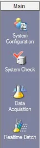
• On the left-hand side toolbar, click on the icon for “Realtime Batch” under the “Main” tab

• Start by adding in the number of rows needed by right-clicking one row, and in the dropdown window, select add a row. This will allow you to add as many rows as needed to run the number of samples.
• In the first row, set the vial number to the location of the first vial you wish to analyze in the tray. Click and drag down to the last row of the “Vial #” column, right-click in the highlighted area, and click “Fill Series” (assuming your samples are all in a row).
• Set the “Sample Name” to something that best identifies your sample to ensure accurate analysis later, making sure it corresponds to the proper vial (the “Sample ID” and “Sample Type” columns may be left blank).
• In the “Method File” column, click in the first box, then click the down arrow to open up a file locator. This is used to open a method to run the samples. Locate the method file to be used and double-click to set it in the batch file. Click and drag the column and select “Fill Down” to set the method file to each row.
• In the “Data File” column, click in the first box, then click the down arrow to open up a file locator. Set the location for the data file to be saved and the name of the sample. This needs to be repeated until each sample has a saved file directory.

Data analysis of samples

• In the “LabSolutions” window, select the “Post Run” tab, then select “Post Run”

• Go to “File” and select “Open Data File”. This will bring up a browser for you to find the data you wish to analyze.
• [1] Select the “Qualitative Peak Integration” icon (it's on the left-hand side of the screen). All peaks of Interest should be labeled at this point.

• [2] Click on each molecular weight specified (only for SIM) and make sure they correspond to an actual peak. [3] Click “OK”
• On the side of the screen select the “Create Compound Wizard” icon.

👉   Select “Integration of TIC”, then hit “Next”.

👉     Input the number of peaks in your spectrum.

👉  Use your controls to label each peak to the corresponding compound within the wizard. At this point you may also enter the concentrations of the standards [1,2].

👉   Move from peak to peak using the up arrow in the wizard [3].

👉  Finish by clicking view on the right side and then click on yes for integration of the peaks again.

• Click on “Save Data and Method File”
• Close the “Postrun Analysis” window completely.
• In the “LabSolutions” window, select the “Post Run” tab, then select “Browser”

• Select “File” \ “Open Method File”
• Select your standards and unknowns for the “data” window and drag them into the center window.
• Select “Peak Integration for All Data”
• Click on each component and write down the concentration levels used in the compound tab on the right.
• Check that all calibration points are good and reject those that are not by unchecking them.

Turning Off the Instrument and Logging off

• Simple excite out of the __ window, it will prompt you asking if you what components you wish to shut off.

ALSO READ: SOP for Operation of Shimadzu LCMS 2020